Most artificial intelligence today is implemented using some form of neural network. In my last two articles, I introduced neural networks and showed you how to build a neural network in Java. The power of a neural network derives largely from its capacity for deep learning, and that capacity is built on the concept and execution of backpropagation with gradient descent. I'll conclude this short series of articles with a quick dive into backpropagation and gradient descent in Java.
Backpropagation in machine learning
It’s been said that AI isn’t all that intelligent, that it is largely just backpropagation. So, what is this keystone of modern machine learning?
To understand backpropagation, you must first understand how a neural network works. Basically, a neural network is a directed graph of nodes called neurons. Neurons have a specific structure that takes inputs, multiplies them with weights, adds a bias value, and runs all that through an activation function. Neurons feed their output into other neurons until the output neurons are reached. The output neurons produce the output of the network. (See Styles of machine learning: Intro to neural networks for a more complete introduction.)
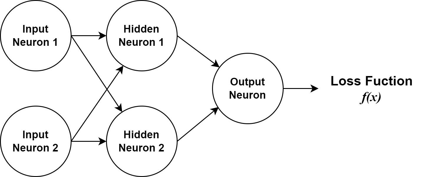
I'll assume from here that you understand how a network and its neurons are structured, including feedforward. The example and discussion will focus on backpropagation with gradient descent. Our neural network will have a single output node, two “hidden” nodes, and two input nodes. Using a relatively simple example will make it easier to see the math involved with the algorithm. Figure 1 shows a diagram of the example neural network.
Figure 1. A diagram of the neural network we'll use for our example.
The idea in backpropagation with gradient descent is to consider the entire network as a multivariate function that provides input to a loss function. The loss function calculates a number representing how well the network is performing by comparing the network output against known good results. The set of input data paired with good results is known as the training set. The loss function is designed to increase the number value as the network's behavior moves further away from correct.
Gradient descent algorithms take the loss function and use partial derivatives to determine what each variable (weights and biases) in the network contributed to the loss value. It then moves backward, visiting each variable and adjusting it to decrease the loss value.
The calculus of gradient descent
Understanding gradient descent involves a few concepts from calculus. The first is the notion of a derivative. MathsIsFun.com has a great introduction to derivatives. In short, a derivative gives you the slope (or rate of change) for a function at a single point. Put another way, the derivative of a function gives us the rate of change at the given input. (The beauty of calculus is that it lets us find the change without another point of reference—or rather, it allows us to assume an infinitesimally small change to the input.)
The next important notion is the partial derivative. A partial derivative lets us take a multidimensional (also known as a multivariable) function and isolate just one of the variables to find the slope for the given dimension.
Derivatives answer the question: What is the rate of change (or slope) of a function at a specific point? Partial derivatives answer the question: Given multiple input variables to the equation, what is the rate of change for just this one variable?
Gradient descent uses these ideas to visit each variable in an equation and adjust it to minimize the output of the equation. That’s exactly what we want in training our network. If we think of the loss function as being plotted on the graph, we want to move in increments toward the minimum of a function. That is, we want to find the global minimum.
Note that the size of an increment is known as the “learning rate” in machine learning.
Gradient descent in code
We’re going to stick close to the code as we explore the mathematics of backpropagation with gradient descent. When the math gets too abstract, looking at the code will help keep us grounded. Let’s start by looking at our Neuron class, shown in Listing 1.
Listing 1. A Neuron class
class Neuron {
    Random random = new Random();
    private Double bias = random.nextGaussian();
    private Double weight1 = random.nextGaussian();
    private Double weight2 = random.nextGaussian();

    public double compute(double input1, double input2){
      return Util.sigmoid(this.getSum(input1, input2));
    }

    public Double getWeight1() { return this.weight1; }
    public Double getWeight2() { return this.weight2; }

    public Double getSum(double input1, double input2){ return (this.weight1 * input1) + (this.weight2 * input2) + this.bias; }
    public Double getDerivedOutput(double input1, double input2){ return Util.sigmoidDeriv(this.getSum(input1, input2)); }
    public void adjust(Double w1, Double w2, Double b){
      this.weight1 -= w1; this.weight2 -= w2; this.bias -= b;
    }
  }
The Neuron class has only three Double members: weight1, weight2, and bias. It also has a few methods. The method used for feedforward is compute(). It accepts two inputs and performs the job of the neuron: multiply each by the appropriate weight, add in the bias, and run it through a sigmoid function.
Before we move on, let's revisit the concept of the sigmoid activation, which I also discussed in my introduction to neural networks. Listing 2 shows a Java-based sigmoid activation function.
Listing 2. Util.sigmoid()
public static double sigmoid(double in){
  return 1 / (1 + Math.exp(-in));
}
The sigmoid function takes the input and raises Euler's number (Math.exp) to its negative, adding 1 and dividing that by 1. The effect is to compress the output between 0 and 1, with larger and smaller numbers approaching the limits asymptotically.
Returning to the Neuron class in Listing 1, beyond the compute() method we have getSum() and getDerivedOutput(). getSum() just does the weights * inputs + bias calculation. Notice that compute() takes getSum() and runs it through sigmoid(). The getDerivedOutput() method runs getSum() through a different function: the derivative of the sigmoid function.
Derivative in action
Now take a look at Listing 3, which shows a sigmoid derivative function in Java. We’ve talked about derivatives conceptually, here's one in action.
Listing 3. Sigmoid derivative
public static double sigmoidDeriv(double in){
  double sigmoid = Util.sigmoid(in);
  return sigmoid * (1 - sigmoid);
}
Remembering that a derivative tells us what the change of a function is for a single point in its graph, we can get a feel for what this derivative is saying: Tell me the rate of change to the sigmoid function for the given input. You could say it tells us what impact the preactivated neuron from Listing 1 has on the final, activated result.
Derivative rules
You might wonder how we know the sigmoid derivative function in Listing 3 is correct. The answer is that we'll know the derivative function is correct if it has been verified by others and if we know the properly differentiated functions are accurate based on specific rules. We don’t have to go back to first principles and rediscover these rules once we understand what they are saying and trust that they are accurate—much like we accept and apply the rules for simplifying algebraic equations.
So, in practice, we find derivatives by following the derivative rules. If you look at the sigmoid function and its derivative, you’ll see the latter can be arrived at by following these rules. For the purposes of gradient descent, we need to know about derivative rules, trust that they work, and understand how they apply. We’ll use them to find the role each of the weights and biases plays in the final loss outcome of the network.
Notation
The notation f prime f’(x) is one way of saying “the derivative of f of x”. Another is:
The two are equivalent:
Another notation you’ll see shortly is the partial derivative notation:
This says, give me the derivative of f for the variable x.
The chain rule
The most curious of the derivative rules is the chain rule. It says that when a function is compound (a function within a function, aka a higher-order function) you can expand it like so:
We’ll use the chain rule to unpack our network and get partial derivatives for each weight and bias.
Putting it in code
We know what the neuron’s members and the sigmoid and its derivatives look like. The last method is adjust(), which takes three arguments. These are values to apply to the weights and bias. It is important to notice that these arguments are subtracted. In gradient descent, we determine what each variable has contributed to the loss and subtract it—remember that we want to minimize the loss. So if the weight/bias has a negative value (that is, it made the loss less), we increase the value by subtracting a negative value. Otherwise, we subtract the positive value. In both cases, the action taken will decrease the loss.
Now how do we make use of these methods? We put the neurons together into a Network object, then train them.
The signatures for the Network class are shown in Listing 4.
Listing 4. Network class overview
class Network {
    double learnRate = .15;
    int epochs = 1000;
    Neuron nHidden1 = new Neuron();
    Neuron nHidden2 = new Neuron();
    Neuron nOutput = new Neuron();

    public Double predict(Double input1, Double input2){...}
         public void train(List<List<Double>> data, List<Double> answers){..}
    public void adjust(Double loss, Double in1, Double in2){...}
}
What Listing 4 shows is the Network's two main abilities: to predict() and to train(). The adjust() method is a convenience method that applies changes to the Neurons. We have three neurons: two hidden neurons and an output. Epochs are the number of training rounds. The learnRate, as discussed before, represents the step size for our gradient descent.
Listing 5. predict()
public Double predict(Double input1, Double input2){
  return nOutput.compute(nHidden1.compute(input1, input2), nHidden2.compute(input1, input2));
}
Listing 5 shows the predict() method. It's very simple but holds the essence of the feedforward process: the hidden nodes take the input and the output node takes the output of the hidden nodes. Now consider the train() method in Listing 6.
Listing 6. Network.train()
public void train(List<List<Double>> data, List<Double> answers){
  double learnRate = .1;
  for (int epoch = 0; epoch < epochs; epoch++){
     for (int i = 0; i < data.size(); i++){
       double in1 = data.get(i).get(0); double in2 = data.get(i).get(1);
       double loss = -2 * (answers.get(i) - this.predict(in1, in2));
       this.adjust(loss, in1, in2);
     }

     if (epoch % 10 == 0){
       List<Double> predictions = data.stream().map( item -> this.predict(item.get(0), item.get(1)) ).collect( Collectors.toList() );
       Double loss = Util.meanSquareLoss(answers, predictions);
       System.out.println("     Epoch " + epoch + "    pred: " + predictions + "     Loss: "+ loss);
      }

    }
  }
The network.train() sets up the loops that handle backpropagation. We loop once for each epoch. Within each epoch we loop over the data and the answer arguments, which are equal-length arraylists. The data is a two-dimensional array. Each element is two data points coming in for, while answers holds the correct output for each pair. We will use this training data to train the network to generate better predictions.
For each data set, we make use of the predict() method to find what the network currently thinks about the input data: this.predict(in1, in2), and then subtract that from the known good answer: answers.get(i).
That part makes sense, but what is the -2 * there? The answer is that we are calculating the derivative of the loss function, which turns out to be -2 * (answers.get(i) - this.predict(in1, in2)).
Our loss function is the mean squared error. Listing 7 shows the Java code for the mean squared error.
Listing 7. Java mean squared error
public static Double meanSquareLoss(List<Double> correctAnswers, List<Double> predictedAnswers){
  double sumSquare = 0;
  for (int i = 0; i < correctAnswers.size(); i++){
    double error = correctAnswers.get(i) - predictedAnswers.get(i);
      sumSquare += (error * error);
    }
  return sumSquare / (correctAnswers.size());
}
Here is the algebra version of Listing 7:
In essence: correct answer minus predicted answer, squared and averaged over the number of data points. In Listing 6, we only have a single data point, so we are just deriving for one answer minus one prediction, squared. We are doing this because it is the first step of walking backward over the network equation and finding the derivatives. Every weight and bias contributes to the overall loss, and so the derived loss will be applied to each of them.
This is the chain rule in effect. Remembering that the chain rule means you break out the compound function into f(g(x)) —> f'(g(x))*g'(x). Well, what we have in the form of the derived loss is the g'(x) for the entire network. It’s actually a multivariable function, but the effect is the same. Our network equation’s final step is to calculate the loss function, so the first step moving backwards in finding derivatives is to differentiate the loss, and multiply that with the f’(g(x). The f’(g(x)) turns out to be different for each weight and bias—it's whatever path the feedforward algorithm took to apply them, but in each case we’ll use the chain rule to further unpack them.
The adjust() method
That’s a lot to digest at first. Let’s return to the code and see how the adjust() method works.
Listing 8. Network.adjust()
public void adjust(Double loss, Double in1, Double in2){
  Double o1W1 = nOutput.getWeight1();
  Double o1W2 = nOutput.getWeight2();

  Double h1Output = nHidden1.compute(in1, in2);
  Double h2Output = nHidden2.compute(in1, in2);

  Double derivedOutput = nOutput.getDerivedOutput(h1Output, h2Output);

  Double derivedH1 = nHidden1.getDerivedOutput(in1, in2);
  Double derivedH2 = nHidden2.getDerivedOutput(in1, in2);

  nHidden1.adjust(
     learnRate * loss * (o1W1 * derivedOutput) * (in1 * derivedH1),
     learnRate * loss * (o1W1 * derivedOutput) * (in2 * derivedH1),
     learnRate * loss * (o1W1 * derivedOutput) * derivedH1);

   nHidden2.adjust(
     learnRate * loss * (o1W2 * derivedOutput) * (in1 * derivedH2),
     learnRate * loss * (o1W2 * derivedOutput) * (in2 * derivedH2),
     learnRate * loss * (o1W2 * derivedOutput) * derivedH2);

   nOutput.adjust(
     learnRate * loss * h1Output * derivedOutput,
     learnRate * loss * h2Output * derivedOutput,
     learnRate * loss * derivedOutput);
   }
}
All the adjust() method needs is the derived loss we just looked at and the two inputs. It begins by saving the weights for the output neuron (o1W1 and o1W2) and the computed outputs for the hidden neurons (h1Output and h2Output). We also grab the derived outputs of all the neurons (derivedOutput, derivedH1, and derivedH2. We need these as a snapshot for when we start making adjustments to the neurons themselves.
It turns out these are the only values we need to find all the derivatives. You’ll see how in a moment.
Look at the nOutput.adjust() method. It takes the learnRate, multiplies it to the derived loss, and then for each weight and the bias finds the partial derivative to modify the value by. For example, the output bias is saying this:
Which we can unpack as the following derivative chain:
Which, if we look at the code for each step, is the following:
-2 * (answers.get(i) - this.predict(in1, in2)) * nOutput.getDerivedOutput(h1Output, h2Output)
That is to say, the derivative of the overall loss based on the prediction versus truth, times the output of the output neuron. The output neuron’s bias is the simplest of the derivations because it is closest to the output and doesn’t directly interact with the other neuron’s input.
Now, to do the actual training we can use the code in Listing 9.
Listing 9. Train()
public void train () {
    Network network = new Network();
    List<List<Double>> data = new ArrayList<List<Double>>();
    data.add(Arrays.asList(-1.0, -5.5));
    data.add(Arrays.asList(-3.5, -2.0));
    data.add(Arrays.asList(5.0, 6.5));
    data.add(Arrays.asList(3.0, 1.5));
    List<Double> answers = Arrays.asList(.98,.95,0.01,0.2);
    network.train(data, answers);
  }
The data array holds the input and the answers hold the correct answers. For the network we have created, the data must pivot on 0. Perhaps this data could be temperatures in celsius and the answers could be the observed chance that a body of water is frozen. In truth, any kind of quantitative input can be massaged into this format.
When we run this code, you’ll see that our loss gradually declines as the network learns to make better predictions that are closer to the answers. Once trained, the network can be used to make predictions against new data sets.
Conclusion
This has been a whirlwind tour of gradient descent. The biggest barrier to understanding backpropagation with gradient descent is the calculus involved. Once that is understood, the overall idea is not hard to grasp and apply in code.
See the following resources to learn more about gradient descent:
- Gradient descent algorithm—a deep dive
- Neural networks and deep learning
- Machine learning for beginners: An introduction to neural networks
- Styles of machine learning: Intro to neural networks
- How to build a neural network in Java