


Putting it in code
We know what the neuron’s members and the sigmoid and its derivatives look like. The last method is adjust(), which takes three arguments. These are values to apply to the weights and bias. It is important to notice that these arguments are subtracted. In gradient descent, we determine what each variable has contributed to the loss and subtract it—remember that we want to minimize the loss. So if the weight/bias has a negative value (that is, it made the loss less), we increase the value by subtracting a negative value. Otherwise, we subtract the positive value. In both cases, the action taken will decrease the loss.
Now how do we make use of these methods? We put the neurons together into a Network object, then train them.
The signatures for the Network class are shown in Listing 4.
Listing 4. Network class overview
class Network {
    double learnRate = .15;
    int epochs = 1000;
    Neuron nHidden1 = new Neuron();
    Neuron nHidden2 = new Neuron();
    Neuron nOutput = new Neuron();

    public Double predict(Double input1, Double input2){...}
         public void train(List<List<Double>> data, List<Double> answers){..}
    public void adjust(Double loss, Double in1, Double in2){...}
}
What Listing 4 shows is the Network's two main abilities: to predict() and to train(). The adjust() method is a convenience method that applies changes to the Neurons. We have three neurons: two hidden neurons and an output. Epochs are the number of training rounds. The learnRate, as discussed before, represents the step size for our gradient descent.
Listing 5. predict()
public Double predict(Double input1, Double input2){
  return nOutput.compute(nHidden1.compute(input1, input2), nHidden2.compute(input1, input2));
}
Listing 5 shows the predict() method. It's very simple but holds the essence of the feedforward process: the hidden nodes take the input and the output node takes the output of the hidden nodes. Now consider the train() method in Listing 6.
Listing 6. Network.train()
public void train(List<List<Double>> data, List<Double> answers){
  double learnRate = .1;
  for (int epoch = 0; epoch < epochs; epoch++){
     for (int i = 0; i < data.size(); i++){
       double in1 = data.get(i).get(0); double in2 = data.get(i).get(1);
       double loss = -2 * (answers.get(i) - this.predict(in1, in2));
       this.adjust(loss, in1, in2);
     }

     if (epoch % 10 == 0){
       List<Double> predictions = data.stream().map( item -> this.predict(item.get(0), item.get(1)) ).collect( Collectors.toList() );
       Double loss = Util.meanSquareLoss(answers, predictions);
       System.out.println("     Epoch " + epoch + "    pred: " + predictions + "     Loss: "+ loss);
      }

    }
  }
The network.train() sets up the loops that handle backpropagation. We loop once for each epoch. Within each epoch we loop over the data and the answer arguments, which are equal-length arraylists. The data is a two-dimensional array. Each element is two data points coming in for, while answers holds the correct output for each pair. We will use this training data to train the network to generate better predictions.
For each data set, we make use of the predict() method to find what the network currently thinks about the input data: this.predict(in1, in2), and then subtract that from the known good answer: answers.get(i).
That part makes sense, but what is the -2 * there? The answer is that we are calculating the derivative of the loss function, which turns out to be -2 * (answers.get(i) - this.predict(in1, in2)).
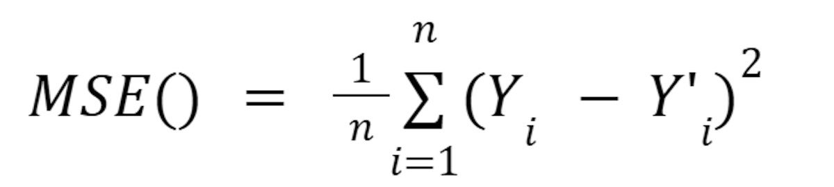
Our loss function is the mean squared error. Listing 7 shows the Java code for the mean squared error.
Listing 7. Java mean squared error
public static Double meanSquareLoss(List<Double> correctAnswers, List<Double> predictedAnswers){
  double sumSquare = 0;
  for (int i = 0; i < correctAnswers.size(); i++){
    double error = correctAnswers.get(i) - predictedAnswers.get(i);
      sumSquare += (error * error);
    }
  return sumSquare / (correctAnswers.size());
}
Here is the algebra version of Listing 7:
 IDG
IDGIn essence: correct answer minus predicted answer, squared and averaged over the number of data points. In Listing 6, we only have a single data point, so we are just deriving for one answer minus one prediction, squared. We are doing this because it is the first step of walking backward over the network equation and finding the derivatives. Every weight and bias contributes to the overall loss, and so the derived loss will be applied to each of them.
This is the chain rule in effect. Remembering that the chain rule means you break out the compound function into f(g(x)) —> f'(g(x))*g'(x). Well, what we have in the form of the derived loss is the g'(x) for the entire network. It’s actually a multivariable function, but the effect is the same. Our network equation’s final step is to calculate the loss function, so the first step moving backwards in finding derivatives is to differentiate the loss, and multiply that with the f’(g(x). The f’(g(x)) turns out to be different for each weight and bias—it's whatever path the feedforward algorithm took to apply them, but in each case we’ll use the chain rule to further unpack them.
The adjust() method
That’s a lot to digest at first. Let’s return to the code and see how the adjust() method works.
Listing 8. Network.adjust()
public void adjust(Double loss, Double in1, Double in2){
  Double o1W1 = nOutput.getWeight1();
  Double o1W2 = nOutput.getWeight2();

  Double h1Output = nHidden1.compute(in1, in2);
  Double h2Output = nHidden2.compute(in1, in2);

  Double derivedOutput = nOutput.getDerivedOutput(h1Output, h2Output);

  Double derivedH1 = nHidden1.getDerivedOutput(in1, in2);
  Double derivedH2 = nHidden2.getDerivedOutput(in1, in2);

  nHidden1.adjust(
     learnRate * loss * (o1W1 * derivedOutput) * (in1 * derivedH1),
     learnRate * loss * (o1W1 * derivedOutput) * (in2 * derivedH1),
     learnRate * loss * (o1W1 * derivedOutput) * derivedH1);

   nHidden2.adjust(
     learnRate * loss * (o1W2 * derivedOutput) * (in1 * derivedH2),
     learnRate * loss * (o1W2 * derivedOutput) * (in2 * derivedH2),
     learnRate * loss * (o1W2 * derivedOutput) * derivedH2);

   nOutput.adjust(
     learnRate * loss * h1Output * derivedOutput,
     learnRate * loss * h2Output * derivedOutput,
     learnRate * loss * derivedOutput);
   }
}
All the adjust() method needs is the derived loss we just looked at and the two inputs. It begins by saving the weights for the output neuron (o1W1 and o1W2) and the computed outputs for the hidden neurons (h1Output and h2Output). We also grab the derived outputs of all the neurons (derivedOutput, derivedH1, and derivedH2. We need these as a snapshot for when we start making adjustments to the neurons themselves.
It turns out these are the only values we need to find all the derivatives. You’ll see how in a moment.
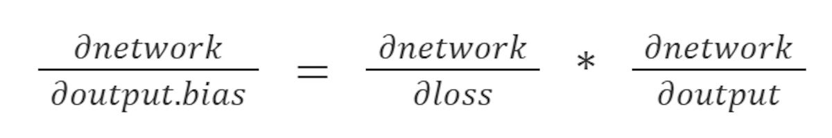
Look at the nOutput.adjust() method. It takes the learnRate, multiplies it to the derived loss, and then for each weight and the bias finds the partial derivative to modify the value by. For example, the output bias is saying this:
 IDG
IDGWhich we can unpack as the following derivative chain:
 IDG
IDGWhich, if we look at the code for each step, is the following:
-2 * (answers.get(i) - this.predict(in1, in2)) * nOutput.getDerivedOutput(h1Output, h2Output)
That is to say, the derivative of the overall loss based on the prediction versus truth, times the output of the output neuron. The output neuron’s bias is the simplest of the derivations because it is closest to the output and doesn’t directly interact with the other neuron’s input.
Now, to do the actual training we can use the code in Listing 9.
Listing 9. Train()
public void train () {
    Network network = new Network();
    List<List<Double>> data = new ArrayList<List<Double>>();
    data.add(Arrays.asList(-1.0, -5.5));
    data.add(Arrays.asList(-3.5, -2.0));
    data.add(Arrays.asList(5.0, 6.5));
    data.add(Arrays.asList(3.0, 1.5));
    List<Double> answers = Arrays.asList(.98,.95,0.01,0.2);
    network.train(data, answers);
  }
The data array holds the input and the answers hold the correct answers. For the network we have created, the data must pivot on 0. Perhaps this data could be temperatures in celsius and the answers could be the observed chance that a body of water is frozen. In truth, any kind of quantitative input can be massaged into this format.
When we run this code, you’ll see that our loss gradually declines as the network learns to make better predictions that are closer to the answers. Once trained, the network can be used to make predictions against new data sets.
Conclusion
This has been a whirlwind tour of gradient descent. The biggest barrier to understanding backpropagation with gradient descent is the calculus involved. Once that is understood, the overall idea is not hard to grasp and apply in code.
See the following resources to learn more about gradient descent: